This post outlines a project I completed for a graduate course on dynamical systems, neural networks, and theoretical neuroscience. I explore how low-rank structure hidden in high-dimensional random connectivity gives rise to spectral outliers: isolated eigenvalues that dominate the macroscopic behavior of otherwise chaotic networks, and how these outliers can serve as early-warning signals for bifurcations in driven recurrent networks. The investigation blends random matrix theory, dynamical mean-field theory, and spectral analysis to make a conceptual ghost quantitative.

It's natural to now step back and ask: what do we already know about chaotic RNNs? How does structure change the story?

The most relevant recent work here is by Rainer Engelken and collaborators. Their NeurIPS 2022 paper developed what they call a non-stationary dynamic mean-field theory (DMFT). Classical DMFT provides us with a way to describe the statistics of large random networks at stationary, but once the network is driven by time-varying inputs, the stationar assumption breaks. Engelken et al. derived a time-resolved closure: equations for the population mean activity, the two-time correlation function of fluctuations, and an auxiliary kernel that makes the system self-consistent. Practically, the framework gives us a tractable way to predict the network's response spectrum, its largest Lyapunov exponent, and even the information-theoretic capacity of the population to transmit signals.

We study a continuous-time rate network with \(N\) units. Each unit carries a synaptic current \(h_i(t)\) and fires at rate \(\phi(h_i)\), with \(\phi(x) = \max(0, x)\) (ReLU). The dynamics are given by the differential equation \[ \tau \frac{d h_i}{dt} = -h_i + \sum_{j=1}^N J_{ij} \phi(h_j) + b I(t) + \xi_i(t). \] Here, \(\tau > 0\) is a membrane/leak timescale, \(J \in \mathbb{R}^{N \times N}\) is a connectivity matrix with balanced mean and random heterogeneity: \[ J_{ij} = -\frac{b}{N}J_0 + \tilde{J}_{ij},\quad \tilde{J}_{ij} \sim \mathcal{N}(0, g^2/N). \] \(b > 0\) tunes the tightness of balance[1] (a stronger \(b\) means stronger recurrent inhibition), \(I(t)\) is a common input (e.g. an OU process with correlation time \(\tau_S\)), and \(\xi_i(t)\) is independent Gaussian noise such that \(\langle \xi_i(t) \xi_i(t') \rangle = \sigma^2 \tau \delta(t - t')\).

We decompose the currents into a population mean and fluctuations: \[ h_i(t) = m(t) + \tilde{h}_i(t),\quad m(t) = \frac{1}{N} \sum_{i=1}^N h_i(t),\quad \langle \tilde{h}_i(t) \rangle = 0. \] Substituting this into the dynamics and using the mean of \(J\) yields two coupled equations \begin{align} \tau \frac{d m}{dt} &= -m -b J_0 \nu(t) + b I(t) \\ \tau \frac{d \tilde{h}_i}{dt} &= -\tilde{h}_i + \sum_{j=1}^N \tilde{J}_{ij} \phi \left(m(t) + \tilde{h}_{ij}(t)\right) + \tilde{\xi}_i(t) \end{align} with the population rate \(\nu(t) = \frac{1}{N} \sum_{i=1}^N \phi\left(m(t) + \tilde{h}_i(t)\right)\). Solving the first equation for \(\nu\) gives the balance equation \[ \nu(t) = \frac{1}{J_0}I(t) - \frac{1}{b J_0} \left(\tau \frac{d m}{dt} + m\right). \] In the tight-balance limit \(b \to \infty\), \(\nu(t)\approx I(t)/J_0\) (linear tracking) and the mean mode acquires an effective timescale \(\tau_{\mathrm{eff}} = \tau/b\). This leads to the first core result.

So far, we've seen the spectral fingerprint: the rank-one mean term adds a single eigenvalue at \(-b\), while the random bulk remains a circular cloud of radius \(g\). This lone outlier is the ghost steering the mean activity. But spectra are only the beginning. The NeurIPS paper showed how this outlier governs the dynamical timescale of the mean. Take a step input and watch the population mean \(m(t)\) relax. The prediction from the balance equation is relatively simple: \[ \tau_{\mathrm{eff}} = \frac{\tau}{b}. \] As \(b\) increases, the mean mode tracks input \(b\)-times faster. In simulations, fitting the exponential decay of \(m(t)\) confirms that the timescale drops as \(1/b\).

Faster mean dynamics suggest wider bandwidth for signal encoding. The DMFT closure makes this intuition quantitative. By treading residuals \(\tilde{h}(t)\) as a Gaussian process with covariance \(c(t, s)\), one can compute the input-output coherence \[ C_{I\nu}(f) = \frac{\left| S_{I\nu}(f)\right|^2}{S_{II}(f) S_{\nu\nu}(f)}, \] Here, \(S_{I\nu}\) is the cross-spectrum of the input and output, and \(S_{II}\), \(S_{\nu\nu}\) are their respective autospectra. The result is that higher balance values keep coherence close to one across higher frequencies, reflecting faster tracking and higher effective bandwidth.

Integrating this coherence function gives us a Gaussian-channel lower bound on the mutual information between the input and output signals. \[ R_{\mathrm{lb}} = -\int\, df \log_2\left(1 - C_{I\nu}(f)\right). \]

This is the one of the headline results of the paper, and our second core finding.

To complete our understanding of this paper, it's worth highlighting a key result from a complementary paper done by Engelken et al. This PLOS paper provides code that shows the same non-stationary DMFT framework was used to compute the largest Lyapunov exponent[2] \(\lambda_1\).

The surprising finding was that common input is poor at surpressing chaos. Because of balance, the common drive enters the mean equation and is canceled by recurrent inhibition. As a result, \(\lambda_1\) only turns negative at very large input amplitudes. Independent input, on the other hand, enters the fluctuation channel directly and is not canceled, so even small amplitudes can suppress chaos.

This closes the loop on what we know. Balance plants a real outlier eigenvalue at \(-b\), accelerates the mean mode, broadens encoding bandwidth, and shapes how chaos can be tamed. But the story doesn't end with theory. The natural next question is experimental: can we go beyond balance and use low-rank structure to predict when a driven network crosses the stability boundary?

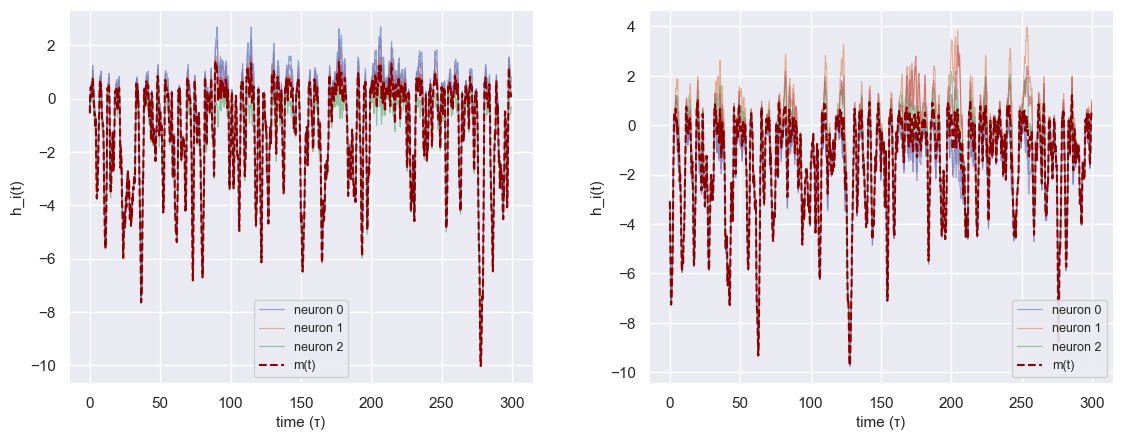
Before pushing into new territory, I wanted to confirm the baseline machinery by reproducing the spectral and DMFT fingerprints under driven chaos. There are three sanity checks:

(i) Trajectories behave as expected as \(g\) increases: fluctuations grow, but remain bounded under strong balance.
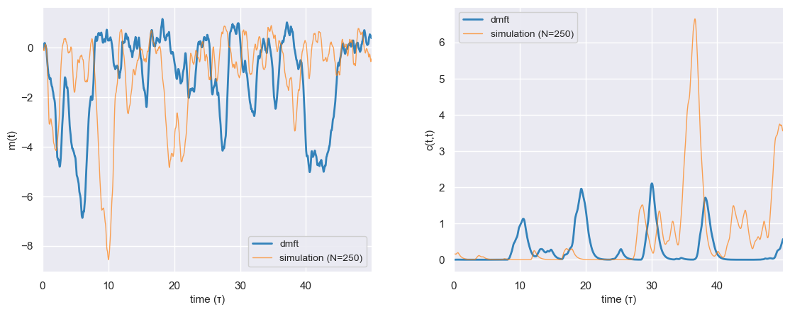
(ii) Non-stationary DMFT qualitatively matches the time-resolved mean \(m(t)\) and variance \(c(t,t)\).
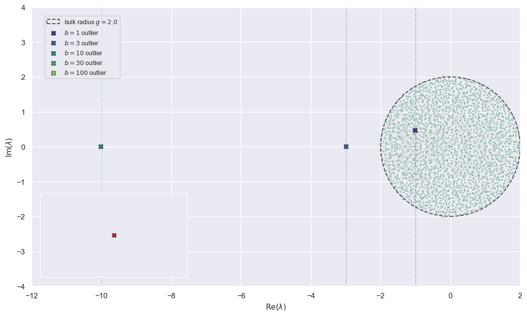
(iii) The spectrum of \(J\) is exactly what it should be: a Ginibre disk of radius \(\approx g\) plus the real outlier at \(-b\).

The spectral check is the one I care about most, because everything that follows is an outlier story. If balance is doing what it claims, then \(J\) should look like: circular bulk + one real spike at \(-b\). And that's exactly what emerges.

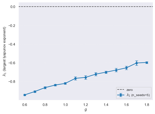
This already hints at something subtle. We often talk as if "the transition to chaos" is a crisp curve in parameter space. But at finite \(N\) and finite simulation horizon, the world is softer: \(\lambda_1\) trends toward zero without crossing. That softness matters once we start using spectral proxies.

The real object controlling stability in a driven system is not the spectrum of \(J\), but the linearization along the trajectory. To move from connectivity outliers to Jacobian outliers, linearize the dynamics: \[ A(t) = -I + J D(t), \qquad D(t) = \mathrm{diag}\!\left(\phi'(h(t))\right), \] where \(D(t)\) is the gain mask that encodes which neurons are active at time \(t\) under ReLU.

If the drive is slow enough, a natural (dangerous) idea is to average: \[ A_{\mathrm{avg}} = -I + J \bar D, \qquad \bar D \approx \mathbb{E}_t[D(t)]. \] This is not a theorem. It's a controlled hallucination: "pretend the driven Jacobian is approximately stationary." But it's the right hallucination if you want an outlier story.

Now we move to a rank-one experiment with a surprisingly useful proxy. Add a rank-one perturbation: \[ J = gW - \frac{b}{N}\mathbf{1}\mathbf{1}^\top + m\,u v^\top, \] with \(u,v\) random unit vectors chosen orthogonal to \(\mathbf{1}\) (so we don't just re-inject another mean mode). The knob is \(m\), the low-rank strength.

The experiment loop is:
(1) Simulate the OU-driven network at fixed \((g,b)\) while sweeping \(m\);
(2) Build \(A_{\mathrm{avg}}\) from the time-averaged gain mask \(\bar D\);
(3) Extract the eigenvalue of \(A_{\mathrm{avg}}\) with largest real part (the "outlier");
(4) Compute \(\lambda_1\) using the Benettin algorithm[3] along the full time-dependent Jacobian.

Here is the punchline: for rank-one structure, there's a scalar proxy for the low-rank outlier: \[ \hat\lambda_{\mathrm{out}}(m) \;\approx\; m\,\bar\alpha - 1, \qquad \bar\alpha = v^\top (\bar D u). \] This is the smallest possible "low-dimensional stability indicator": one number extracted from \(\bar D\). If \(\hat\lambda_{\mathrm{out}}\) tracks \(\lambda_1\), then we've learned something structural: the low-rank mode is steering the boundary.

What I find satisfying is not that the curves coincide. They don't. What matters is that they move together. As \(m\) increases, the outlier of \(A_{\mathrm{avg}}\) slides right; the scalar proxy slides with it; and \(\lambda_1(m)\) trends toward zero. In the parameter range I explored, everything stayed stable (no actual crossing), but the alignment is the central sanity check:

The low-rank mode appears to be the first macroscopic "handle" on stability, even under drive.

There is a clean reason to be suspicious about where the proxy fails, and why that's not a defeat. Stability in a driven system is governed by the time-ordered product of Jacobians, a non-commutative object. A single averaged matrix \(A_{\mathrm{avg}}\) cannot capture non-normal transient growth[4], nor can it see fast input regimes. This is why, in exploratory phase-slices at larger \(g\) and \(m\), the proxy can become positive while sparse \(\lambda_1\) checks remain negative.

I don't see this as failure. I see it as a map: it tells us exactly where the quasi-stationary picture breaks.

The honest endgame for making the ghost quantitative is not a proxy. It's a full low-rank, non-stationary DMFT: a time-resolved closure not just for the mean \(m(t)\) and covariance \(c(t,s)\), but also for the overlap variables \(\kappa(t)\) that carry low-rank structure. At rank \(R\), these overlaps live in \(\mathbb{R}^R\), and they are the natural "order parameters" of the structured mode.

Once you have \((m,c,\kappa)\), the stability question becomes low-dimensional again: linearize the overlap update map and track when the maximal real part crosses zero. That would turn the ghost into a genuine stability boundary, not a heuristic.

The path forward is clear. Solve the low-rank NS-DMFT equations numerically (including overlaps) instead of relying on trajectory averages. Map the \((g,m)\) plane at larger \(N\) and longer horizons until \(\lambda_1\) actually crosses zero. Move beyond rank-one: \(R>1\) structure introduces multiple outliers, and the question becomes which one controls the bifurcation. Stress test the assumptions: rapid drive, large \(g\), non-normality, different nonlinearities.

What began as a study of spectral outliers in balanced networks ended in a concrete bridge between finite-rank matrix theory and the stability of non-autonomous dynamical systems. The ghost is no longer just a metaphor. It's a quantifiable signal, a low-dimensional order parameter hidden inside high-dimensional chaos. I'm grateful to Rainer Engelken for his guidance throughout this project; the full technical report is available here.