← blog

a ghost in the machine

09.28.2025

This post will be the first of $N$ in a series outlining a project I am completing for a $graduate course$ on dynamical systems, neural networks, and theoretical neuroscience. Specifically, I will be exploring how low-rank structure hidden in high-dimensional random connectivity gives rise to spectral outliers: isolated eigenvalues that dominate the macroscopic behavior of otherwise chaotic networks. We will pull ideas from theories of random matrices, dynamical mean fields, and free probability to understand these phenomena.

It's natural to now step back and ask: what do we already know about chaotic RNNs? How does structure change the story?

The most relevant recent work here is by Rainer Engelken and collaborators. Their NeurIPS 2022 paper developed what they call a non-stationary dynamic mean-field theory (DMFT). Classical DMFT provides us with a way to describe the statistics of large random networks at stationary, but once the network is driven by time-varying inputs, the stationar assumption breaks. Engelken et al. derived a time-resolved closure: equations for the population mean activity, the two-time correlation function of fluctuations, and an auxiliary kernel that makes the system self-consistent. Practically, the framework gives us a tractable way to predict the network's response spectrum, its largest Lyapunov exponent, and even the information-theoretic capacity of the population to transmit signals.

We study a continuous-time rate network with $N$ units. Each unit carries a synaptic current $h_i(t)$ and fires at rate $\phi(h_i)$, with $\phi(x) = \max(0, x)$ (ReLU). The dynamics are given by the differential equation \[ \tau \frac{d h_i}{dt} = -h_i + \sum_{j=1}^N J_{ij} \phi(h_j) + b I(t) + \xi_i(t). \] Here, $\tau > 0$ is a membrane/leak timescale, $J \in \mathbb{R}^{N \times N}$ is a connectivity matrix with balanced mean and random heterogeneity: \[ J_{ij} = -\frac{b}{N}J_0 + \tilde{J}_{ij},\quad \tilde{J}_{ij} \sim \mathcal{N}(0, g^2/N). \] $b > 0$ tunes the tightness of balance (a stronger $b$ means stronger recurrent inhibition), $I(t)$ is a common input (e.g. an OU process with correlation time $\tau_S$), and $\xi_i(t)$ is independent Gaussian noise such that $\langle \xi_i(t) \xi_i(t') \rangle = \sigma^2 \tau \delta(t - t')$. We decompose the currents into a population mean and fluctuations: \[ h_i(t) = m(t) + \tilde{h}_i(t),\quad m(t) = \frac{1}{N} \sum_{i=1}^N h_i(t),\quad \langle \tilde{h}_i(t) \rangle = 0. \] Substituting this into the dynamics and using the mean of $J$ yields two coupled equations \begin{align} \tau \frac{d m}{dt} &= -m -b J_0 \nu(t) + b I(t) \\ \tau \frac{d \tilde{h}_i}{dt} &= -\tilde{h}_i + \sum_{j=1}^N \tilde{J}_{ij} \phi \left(m(t) + \tilde{h}_{ij}(t)\right) + \tilde{\xi}_i(t) \end{align} with the population rate $\nu(t) = \frac{1}{N} \sum_{i=1}^N \phi\left(m(t) + \tilde{h}_i(t)\right)$. Solving the first equation for $\nu$ gives the balance equation \[ \nu(t) = \frac{1}{J_0}I(t) - \frac{1}{b J_0} \left(\tau \frac{d m}{dt} + m\right). \] In the tight-balance limit $b \to \infty$, $\nu(t)\approx I(t)/J_0$ (linear tracking) and the mean mode acquires an effective timescale $\tau_{\mathrm{eff}} = \tau/b$. This leads to the first core result.

"Balance speeds up the population mean by a factor of $b$."

So far, we've seen the spectral fingerprint: the rank-one mean term adds a single eigenvalue at $-b$, while the random bulk remains a circular cloud of radius $g$. This lone outlier is the ghost steering the mean activity. But spectra are only the beginning. The NeurIPS paper showed how this outlier governs the dynamical timescale of the mean. Take a step input and watch the population mean $m(t)$ relax. The prediction from the balance equation is relatively simple: \[ \tau_{\mathrm{eff}} = \frac{\tau}{b}. \] As $b$ increases, the mean mode tracks input $b$-times faster. In simulations, fitting the exponential decay of $m(t)$ confirms that the timescale drops as $1/b$.

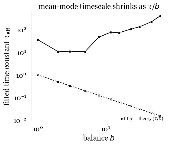
Figure 1: Balance-induced speedup of population dynamics. The effective timescale τ_eff of the population mean decreases as 1/b, demonstrating how tighter balance leads to faster tracking of external inputs.

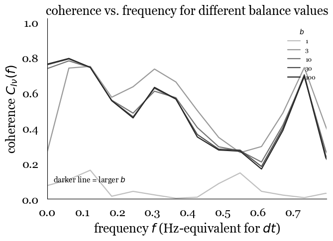
Faster mean dynamics suggest wider bandwidth for signal encoding. The DMFT closure makes this intuition quantitative. By treading residuals $\tilde{h}(t)$ as a Gaussian process with covariance $c(t, s)$, one can compute the input-output coherence \[ C_{I\nu}(f) = \frac{\left| S_{I\nu}(f)\right|^2}{S_{II}(f) S_{\nu\nu}(f)}, \] Here, $S_{I\nu}$ is the cross-spectrum of the input and output, and $S_{II}$, $S_{\nu\nu}$ are their respective autospectra. The result is that higher balance values keep cohere close to one across higher frequencies, reflecting faster tracking and higher effective bandwidth

Figure 2: Input-output coherence as a function of frequency and balance. Higher balance values maintain coherence close to one across higher frequencies, demonstrating improved signal tracking and increased effective bandwidth.

Integrating this coherence function gives us a Gaussian-channel lower bound on the mutual information between the input and output signals. \[ R_{\mathrm{lb}} = -\int\, df \log_2\left(1 - C_{I\nu}(f)\right). \]

This is the one of the headline results of the paper, and our second core finding.

"The information rate grows nearly linearly with balance until it saturates at the bandwidth limit imposed by the input itself."

Figure 3: Information rate scaling with balance parameter. The mutual information between input and output grows nearly linearly with balance until saturating at the bandwidth limit of the input signal.

To complete our understanding of this paper, it's worth highlighting a key result from a complementary paper done by Engelken et al. This PLOS paper provides code that shows the same non-stationary DMFT framework was used to compute the largest Lyapunov exponent $\lambda_1$.

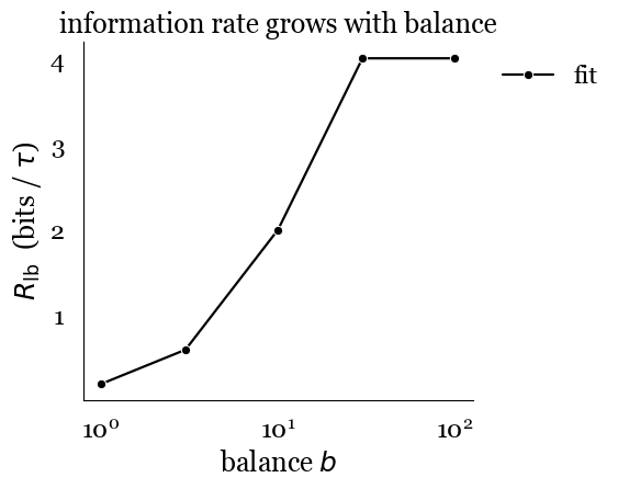
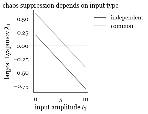
The surprising finding was that common input is poor at surpressing chaos. Because of balance, the common drive enters the mean equation and is canceled by recurrent inhibition. As a result, $\lambda_1$ only turns negative at very large input amplitudes. Input independent, on the other hand, enters the fluctuation channel directly and is not canceled, so even small amplitudes can suppress chaos.

Lyapunov exponent suppression by common vs independent input

Figure 4: Chaos suppression by input type. Common input (top) requires large amplitudes to suppress chaos due to balance cancellation, while independent input (bottom) can suppress chaos even at small amplitudes by directly affecting fluctuation dynamics.

This closes the loop on what we know. Balance plants a real outlier eigenvalue at $-b$, accelerates the mean mode, broadens encoding bandwidth, and shapes how chaos can be tamed. In the next post, I'll go beyond balance and introduce low-rank perturbations \[ S = \sum_{k=1}^R m_k u_k v_k^T, \] on top of the random bulk. Each term creates a new spectral outlier $\lambda_{\mathrm{out}}$. My goal is to show that the real part of these outliers predicts exactly when the network bifurcates (from a fixed point to Hopf oscillations to chaos.) The hope is to expend DMFT with low-rank order parameters and make the ghost in the machine fully quantitative.