Long before Markov chains became algorithms, Andrey Markov used literature to show why dependence need not destroy statistical regularity. In 1913, he worked through the first 20,000 letters of Pushkin's Eugene Onegin, classifying each one as a vowel or consonant and counting which class followed which. The next letter's class depended strongly on the one before it, yet the empirical frequencies still settled into a stable pattern. Here was the essential tension: a process could remember its present state without remaining hostage to its distant past.

Animate one sequence Current class: consonant

After a consonant, a vowel came next 66.3% of the time in Markov's sample.

At that point, the chain was mainly a mathematical object, useful for studying dependent trials. Three decades later, the computational problems at Los Alamos gave it a different role. Stanislaw Ulam proposed simulation when direct combinatorics became unmanageable, John von Neumann connected the idea to neutron transport, and the group around Nicholas Metropolis turned repeated random transitions into a general sampling method. The 1953 Metropolis paper supplied the decisive rule: propose a local move, then accept or reject it so that the long-run distribution is the one we wanted all along.¹

This recipe makes a chain easy to run, but it leaves open the question that determines whether the resulting computation is trustworthy: how long should we wait? If the chain remembers its starting point for exponentially many steps, then a long stream of samples can still describe the transient rather than the target distribution. More samples do not repair that bias when they all come from the same unmixed regime. A useful Monte Carlo method therefore needs a certificate that the memory of the initial state disappears quickly.

For the matching chains in this post, that certificate eventually becomes a traffic argument. We imagine demand moving between pairs of states, ask which transition is forced to carry the heaviest load, and translate the answer into a spectral bound. The classical proof routes this traffic across the entire state space, which is natural but expensive. A 2025 result of Chen, Feng, Ju, Miao, Yin, and Zhang improves a bound that had stood since 1989 by retaining the old routes while changing the scale at which they are used: transport locally, then lift the resulting inequalities to the full chain.

I. The Chain Behind the Story

To see where a proof can lose time, we first need the chain it is trying to control. Fix a graph \(G=(V,E)\), and let a matching \(M\subseteq E\) be a set of edges with no shared endpoints. The monomer–dimer distribution assigns \[ \mu(M)=\frac{\lambda^{|M|}}{Z_G(\lambda)}, \qquad Z_G(\lambda)=\sum_{M'\in\mathcal M_G}\lambda^{|M'|}, \] where \(\lambda>0\) controls how strongly the distribution favors larger matchings. The normalizing constant \(Z_G(\lambda)\) is a sum over every matching in the graph, so calculating it directly quickly becomes impractical. Sampling from \(\mu\) gives an indirect route to that partition function, and through it to several approximate-counting problems built from matchings.

The Jerrum–Sinclair chain explores this enormous family by touching only one randomly chosen graph edge at a time. Depending on the current matching, it may add the edge, remove it, or exchange it with a conflicting matched edge, after which a Metropolis acceptance step corrects for the weights in \(\mu\). Each update is deliberately modest: the matching constraint is never violated, while repeated updates can eventually connect the whole state space. The construction makes \(\mu\) stationary; the harder question is how quickly the chain begins to look stationary from an arbitrary start.

Let \(P\) denote the lazy version of this chain, which occasionally stays put to avoid periodic behavior. Its mixing time is \[ \tau_{\mathrm{mix}}(\epsilon) =\min\left\{t:\max_{M\in\mathcal M_G} \left\|P^t(M,\cdot)-\mu\right\|_{\mathrm{TV}}\leq\epsilon\right\}. \] In words, this is the worst-case number of steps required before the chain lies within \(\epsilon\) of stationarity. Jerrum and Sinclair's analysis, later sharpened by Sinclair, gives \(O_\lambda(mn^2\log n)\) for an \(n\)-vertex, \(m\)-edge graph. That polynomial guarantee was strong enough to power the first general approximation results, but its factor of \(n^2\) also survived decades of improvements elsewhere in the theory. The 2025 result replaces the graph-dependent core of the bound by \[ \tau_{\mathrm{mix}}=\widetilde O_\lambda(\Delta^2m), \] where \(\Delta\) is the maximum degree. On bounded-degree graphs, the old \(n^2\) dependence disappears. Understanding why requires following the proof closely enough to see where it began paying for distance that the chain itself did not need to travel.

II. Mixing Is a Traffic Problem

The first conceptual move is to stop watching one sample path and instead look at all possible transitions at once. Consider any finite reversible chain with state space \(\Omega\), transition matrix \(P\), and stationary distribution \(\pi\). Its transition graph has a directed edge \(e=(u,v)\) whenever \(P(u,v)>0\), and the stationary flow through that edge is \[ Q(e)=\pi(u)P(u,v). \] This quantity behaves like a capacity. It is the probability that a chain already at stationarity crosses \(e\) in one step, so a transition with small \(Q(e)\) is a narrow road through the state space.

We now ask this road network to carry a deliberately demanding traffic pattern. A canonical-path system assigns a route \(\gamma_{x,y}\) to every ordered pair \((x,y)\), while \(\pi(x)\pi(y)\) plays the role of demand that must travel from \(x\) to \(y\). Once every pair has been routed, the edge congestion is the largest load-to-capacity ratio, \[ \rho=\max_e\frac{1}{Q(e)} \sum_{(x,y):\,e\in\gamma_{x,y}}\pi(x)\pi(y). \] A small \(\rho\) says that the prescribed traffic can cross the transition graph without overwhelming any one edge. The point of the construction is that a statement about these artificial routes becomes a statement about the original chain.

The theorem turns routed traffic into conductance, but conductance is still one step removed from mixing. Cheeger's inequality closes that gap by giving \(\lambda_1\geq\Phi^2/2\), so the two bounds imply \[ \lambda_1\geq\frac{1}{8\rho^2}, \] while the spectral gap controls the mixing time through \[ \tau_{\mathrm{mix}}(\epsilon) \leq\frac{1}{\lambda_1} \left(\log\frac{1}{\pi_{\min}}+\log\frac{1}{\epsilon}\right). \] We have reduced a question about convergence from every starting state to a load calculation on a set of chosen routes. That reduction is powerful because it is constructive, but the quality of the certificate now depends on both the routes and the inequalities used to interpret them.

The Boolean hypercube gives a clean view of both the method and its slack. Let \(\Omega=\{0,1\}^n\), and at each step either stay put or flip one uniformly chosen bit. If we route \(x\) to \(y\) by flipping their differing coordinates in numerical order, then every transition has capacity \(1/(n2^{n+1})\), while \(2^{n-1}\) ordered pairs use each directed edge. Therefore \[ \rho=\frac{2^{n-1}\cdot2^{-2n}}{1/(n2^{n+1})}=n, \] which certifies \(\lambda_1\geq1/(8n^2)\) and \(\tau_{\mathrm{mix}}(\epsilon)=O(n^3+n^2\log(1/\epsilon))\). The exact gap is \(1/n\), and the true mixing time is \(\Theta(n\log(n/\epsilon))\), so the traffic proof has found the right qualitative story while losing polynomial factors in the translation. There are two places to look for that loss: the routes may concentrate demand unnecessarily, or the passage from their congestion to the spectral gap may be too indirect.

III. A Global Proof Pays Twice

The hypercube calculation separates the proof into two decisions that are easy to conflate. First, we choose how every pair sends demand through the state space. Then, after the traffic has been routed, we choose an inequality that converts its worst congestion into decay of the chain. Each decision can introduce its own loss, and the historical improvements attacked them in that order.

Fractional flow changes the first decision by giving each pair more than one road. A deterministic system commits all of \(\pi(x)\pi(y)\) to a single path, even when several routes are equally natural, whereas a fractional system can divide that demand among them. Sinclair showed that the conductance argument survives this relaxation with \(\rho_f\) in place of \(\rho\). The proof no longer has to create a bottleneck merely because an arbitrary tie-breaking rule sent too many pairs in the same direction.

fixed routes fractional flow

The small matching space above makes this freedom visible without hiding the calculation behind asymptotics. Averaging over valid shortest toggle orders lowers the maximum congestion from \(61.1\) to \(39.5\), even though the resulting flow has not been optimized. The improvement comes from avoiding an artificial commitment: when many equally short routes exist, a fixed order can overload one transition for no reason intrinsic to the chain.

In a general graph, matchings come with exactly the structure needed to exploit the same idea. For two matchings \(M\) and \(M'\), the symmetric difference \(M\triangle M'\) decomposes into alternating paths and even cycles, and a route from one matching to the other can unwind those components one at a time. Averaging over the valid component orders spreads demand that a fixed order would concentrate. This geometric fact, more than any special algebra of the partition function, is what allowed the flow method to power the approximate-counting program for matchings and permanents.²

IV. The Length Tax

Fractional flow improves the routes, but it does not change the square introduced when conductance passes through Cheeger's inequality. Diaconis and Stroock addressed this second loss by bypassing conductance and applying the paths directly to the Poincaré inequality. To see what changes, it helps to place the chain's local and global variation beside each other.

The Dirichlet form measures the variation visible across one legal transition, \[ \mathcal E(f,f)=\tfrac12\sum_{x,y}\pi(x)P(x,y)(f(x)-f(y))^2 =\sum_{e=\{u,v\}}Q(e)(f(u)-f(v))^2, \] whereas the stationary variance measures the variation between arbitrary pairs of states, \[ \operatorname{Var}_\pi(f) =\tfrac12\sum_{x,y}\pi(x)\pi(y)(f(x)-f(y))^2. \] The spectral gap is the optimal ratio between these two scales, \[ \lambda_1=\inf_{f\ \mathrm{nonconstant}} \frac{\mathcal E(f,f)}{\operatorname{Var}_\pi(f)}. \] A path enters by expressing each global difference as a sum of local differences. The spectral problem has again become a routing problem, now without the detour through a boundary cut.

This direct route replaces the quadratic congestion term from Cheeger with \(\rho\ell_{\max}\), and a fractional version can average path length against the flow rather than charging every pair the absolute worst case. The gain is substantial when demand can be distributed across paths whose lengths remain small relative to their congestion. Yet the proof has not made distance disappear; it has merely exposed the price of distance as an explicit factor.

For the classical matching construction, that price can still be \(\Theta(n)\), because two arbitrary matchings may differ along components spanning a linear fraction of the graph. The Poincaré bound records the full length of those routes and leads back to the \(O_\lambda(mn^2\log n)\) mixing time stated earlier. By 1992, the flow could split across routes and the spectral conversion was direct, but the proof was still comparing arbitrary pairs across the entire state space. Its remaining loss came from the global scale of the comparison itself.

V. Why the Bound Stayed Put

This is where the classical argument seemed to run out of room. Canonical paths tolerate general graphs because they build an explicit transport plan and can follow whatever alternating geometry the instance provides. The same explicitness becomes a liability when the plan must connect every global pair, since far-apart matchings force long routes even if the chain's slow behavior is governed by much more local comparisons.

High-dimensional-expander methods approach the problem from the opposite direction. They condition on part of the configuration, prove that the remaining small walks mix, and then lift those local estimates to the global chain, a route that can produce nearly linear bounds when the degree is bounded. For the monomer–dimer model on general graphs, however, the available local analysis accumulated correlation decay too aggressively as \(\Delta\) grew. Locality removed the long paths, but the lifting step paid elsewhere.

The two proof traditions were losing complementary factors. The classical method had a robust transport plan whose routes were too long, while the local method worked at the right scale but accumulated decay too harshly. A sharper argument would have to borrow the useful part of each: explicit transport from canonical paths, and nearby comparisons from local-to-global analysis.

VI. Route Locally, Lift Globally

Chen and collaborators make precisely this exchange. After fixing a partial assignment of edge variables, choose one remaining edge \(e\) and compare the two conditional distributions obtained by forcing \(e\) to be absent or present. These distributions are coupled so that a sampled pair \((X,Y)\) differs only along the alternating path or cycle containing \(e\). The classical matching path can then transport mass between \(X\) and \(Y\), but it travels only across the component created by this local disagreement. The old geometry survives; the demand it carries has become local.

previous next 1 / 5

Following the stages in the figure reveals why both halves are necessary. The coupled transport proves local Poincaré and log-Sobolev inequalities without paying for a route across the full configuration space.³ The second half of the argument then lifts those inequalities globally while accumulating correlation decay additively. Local transport removes the \(\Theta(n)\) path-length loss, and additive lifting avoids the exponential dependence that had limited earlier local analyses.

For constant \(\lambda\), the resulting mixing time is \(\widetilde O_\lambda(\Delta^2m)\). The improvement is largest when \(\Delta\ll n\), while the bound returns to the old scale as \(\Delta\) approaches \(n\). More revealing than the formula itself is the change in the proof's unit of work. Global convergence is no longer certified by routing between every distant pair; it is assembled from transports between nearby conditional distributions.

This is the slow art in fast mixing. The 1989 path construction already contained the right geometric idea, but its global use asked that idea to solve a more expensive transport problem than the proof ultimately needed. Thirty-six years later, the successful move was neither to discard those paths nor to search for a completely different chain, but to place the paths inside a local-to-global argument. When global routes are too long, condition until the comparison becomes local, prove the functional inequality there, and let the lifting theorem carry it back to the full chain.

---

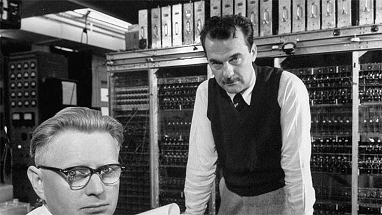
1. Metropolis stayed at Los Alamos for most of his career, and the photo at the top of this post is from his time there. The Metropolis algorithm was, by his own account, mostly the Rosenbluths' and Tellers' work, but the name stuck.
2. A Fully Polynomial Randomized Approximation Scheme is a randomized algorithm that returns a \((1\pm\epsilon)\)-approximation in time polynomial in the input size and \(1/\epsilon\).
3. The log-Sobolev constant controls entropy decay and can produce sharper mixing bounds than the spectral gap. Chen et al. prove both local Poincaré and local log-Sobolev inequalities before lifting them.

References

1. Faster Mixing of the Jerrum–Sinclair Chain
   Chen, X., Feng, W., Ju, Z., Miao, T., Yin, Y. and Zhang, X. (2025).
2. Approximating the Permanent
   Jerrum, M. and Sinclair, A. (1989).
3. Improved Bounds for Mixing Rates of Markov Chains and Multicommodity Flow
   Sinclair, A. (1992).
4. Geometric Bounds for Eigenvalues of Markov Chains
   Diaconis, P. and Stroock, D. (1991).
5. Equation of State Calculations by Fast Computing Machines
   Metropolis, N., Rosenbluth, A. W., Rosenbluth, M. N., Teller, A. H. and Teller, E. (1953).
6. Markov Chains and Mixing Times (2nd ed.)
   Levin, D. A., Peres, Y. and Wilmer, E. L. (2017).
7. Bounds on the \(L^2\) Spectrum for Markov Chains and Markov Processes
   Lawler, G. F. and Sokal, A. D. (1988).
8. A Polynomial-Time Approximation Algorithm for the Permanent of a Matrix with Nonnegative Entries
   Jerrum, M., Sinclair, A. and Vigoda, E. (2004).
9. Log-Concave Polynomials II: High-Dimensional Walks and an FPRAS for Counting Bases of a Matroid
   Anari, N., Liu, K., Oveis Gharan, S. and Vinzant, C. (2019).