fault lines in phase space
11.28.2025
In the previous post, we saw how balance creates a single spectral outlier at \(-b\) that governs mean dynamics, accelerates the population mode, and broadens encoding bandwidth. But what if we go beyond a single rank-one term? What happens when we add structured, low-rank perturbations to the random bulk?
This post develops a complete theoretical framework showing how low-rank structure creates spectral outliers that predict phase transitions. We'll build the theory step by step, then validate it with numerical results. The key insight: the real part of these outliers acts as a "fault line" in phase space, marking where the network transitions from fixed points to oscillations to chaos.
beyond balance: introducing low-rank perturbations
We extend our connectivity matrix to include structured, low-rank terms: \[ J = gW - \frac{b}{N}J_0 \mathbf{1}\mathbf{1}^T + S \] where:
- \(gW\): the random bulk, with \(W\) a real Ginibre matrix scaled by \(1/\sqrt{N}\), giving bulk radius \(g\)
- \(-\frac{b}{N}J_0 \mathbf{1}\mathbf{1}^T\): the rank-one mean term (balance, from the previous post)
- \(S = \sum_{k=1}^R m_k u_k v_k^T = UMV^T\): the new low-rank perturbation
Each term \(m_k u_k v_k^T\) creates structure: a rank-one pattern in connectivity. The parameters are:
- \(R\): the number of low-rank modes (the rank)
- \(m_k\): the strength of the \(k\)-th mode
- \(u_k, v_k \in \mathbb{R}^N\): deterministic unit vectors defining the structure
Why low-rank? Biologically, structured connectivity patterns appear in feature selectivity, task-specific circuits, and learned representations. Computationally, each rank-one term can encode a computational mode. Mathematically, finite-rank perturbations on random matrices create isolated outliers that we can track analytically.
spectral theory: finite-rank outliers on random matrices
The spectral picture now has three components:
- Random bulk: Circular law with radius \(g\) (from \(gW\)), eigenvalues uniformly distributed in a disk
- Balance outlier: Real eigenvalue at \(-b\) (from the rank-one mean term)
- Low-rank outliers: Each term \(m_k u_k v_k^T\) can create an outlier \(\lambda_{\mathrm{out}}^{(k)}\)
To find these outliers, we use a powerful tool: the matrix determinant lemma. For any invertible matrix \(A\) and rank-\(R\) perturbation \(UV^T\), \[ \det(A + UV^T) = \det(A) \det(I + A^{-1}UV^T) \] This reduces an \(N \times N\) determinant to an \(R \times R\) determinant—a massive simplification.
Applying this to our connectivity, for \(J = gW + S\) where \(S = UMV^T\) with \(M = \mathrm{diag}(m_1, \ldots, m_R)\), we get: \[ \det(zI - (gW + S)) = \det(zI - gW) \det(I_R - M\mathcal{R}_W(z)) \] where \(\mathcal{R}_W(z) = V^T(zI - gW)^{-1}U\) is the resolvent projected onto the structured subspaces. Any eigenvalue \(z\) with \(\det(zI - gW) \neq 0\) must satisfy: \[ \det(I_R - M\mathcal{R}_W(z)) = 0 \]
Now comes the key step: the isotropic resolvent limit. For \(|z| > g\) (outside the bulk), the circular law implies that for any fixed \(U, V\) with \(R = \mathcal{O}(1)\), \[ \mathcal{R}_W(z) = V^T(zI - gW)^{-1}U \xrightarrow[N \to \infty]{\text{a.s.}} -z^{-1}V^TU \] Outside the bulk, the resolvent looks like \(-z^{-1}I\)—this is the isotropic limit.
Substituting this into our determinant condition gives: \[ \det(I_R + \frac{M}{z}V^TU) = 0 \iff \det(zI_R + M V^TU) = 0 \]
Theorem (Finite-Rank Outliers): Any limit point \(z\) of an eigenvalue of \(gW + S\) with \(|z| > g\) satisfies \[ \det(zI_R + M V^TU) = 0 \]
In the special case where \(V^TU = \mathrm{diag}(\alpha_1, \ldots, \alpha_R)\) (diagonal overlaps), this simplifies dramatically: \[ z_k = -m_k \alpha_k, \quad k = 1, \ldots, R \] Each \(z_k\) appears as an isolated outlier if \(|z_k| > g\); otherwise, it's absorbed by the Ginibre bulk.
For the full connectivity \(J = gW - \frac{b}{N}J_0 \mathbf{1}\mathbf{1}^T + S\), we stack the rank-one mean and rank-\(R\) spike together. When \(\mathbf{1}\) is orthogonal to \(\{U, V\}\) and \(V^TU\) is diagonal, the outliers decouple to the union of \(-b\) (from balance) and \(-m_k\alpha_k\) (from low-rank structure). This gives us a closed-form predictor for all isolated eigenvalues.
extending dmft: low-rank order parameters
The spectral theory tells us where outliers appear, but to understand dynamics, we need to extend the non-stationary DMFT framework. The challenge: how do we incorporate low-rank structure into the mean-field equations?
The answer lies in low-rank overlaps. For connectivity \(J = gW - \frac{b}{N} \mathbf{1}\mathbf{1}^T + S\) with \(S = \sum_{k=1}^R m_k u_k v_k^T\), the structured drive to neuron \(i\) is: \[ \mu_i^{\mathrm{struct}}(t) = \sum_{k=1}^R m_k u_{k,i} \kappa_k(t) \] where the overlaps are: \[ \kappa_k(t) = \frac{1}{\sqrt{N}} v_k^T \phi(h(t)) \] These capture how much the network "projects" onto each structured mode.
Under exchangeability and the Gaussian reduction for fluctuations \(\tilde{h}(t)\), the \(R\) overlaps obey a self-consistency: \[ \kappa(t) = C M \chi(t) \] where:
- \(C = \frac{1}{N}V^TU \in \mathbb{R}^{R \times R}\) (overlap matrix between structure vectors)
- \(M = \mathrm{diag}(m_1, \ldots, m_R)\)
- \(\chi(t) = \mathbb{E}_{u,\tilde{h}}[u \phi(m(t) + u^T M \kappa(t) + \tilde{h}(t))]\)
- \(\tilde{h}(t) \sim \mathcal{N}(0, c(t,t))\) (Gaussian fluctuations from random bulk)
The mean and covariance equations retain their baseline form but with a shifted mean: \[ \tau \frac{dm}{dt} = -m(t) - bJ_0 \nu(t) + bI(t) \] where \(\nu(t) = \mathbb{E}[\phi(m(t) + u^T M \kappa(t) + \tilde{h}(t))]\), and the covariance equations are evaluated with the same shift inside the moment \(q(t,s)\).
To understand stability, we linearize the overlap map \(\kappa \mapsto C M \chi(\kappa)\) around the trajectory. This gives: \[ \delta \kappa(t) = J_{\mathrm{red}}(t) \delta \kappa(t) \] where the reduced Jacobian is: \[ J_{\mathrm{red}}(t) = C M A(t) \] with \[ A_{ab}(t) = \mathbb{E}_{u,\tilde{h}}[u_a u_b \phi'(m(t) + u^T M \kappa(t) + \tilde{h}(t))] \]
The \(R\) instantaneous "outliers" are the eigenvalues of \(J_{\mathrm{red}}(t)\). The network undergoes a macroscopic transition when: \[ \max_k \mathrm{Re}(\lambda_k(J_{\mathrm{red}}(t))) = 0 \] This is the crossing criterion—it marks the fault line where stability is lost.
When \(V^TU\) is diagonal and \(u, v\) are orthogonal to \(\mathbf{1}/\sqrt{N}\), then \(C = \mathrm{diag}(\alpha_1, \ldots, \alpha_R)\) and \(J_{\mathrm{red}}(t)\) is diagonal, yielding \(\lambda_k(t) = m_k \alpha_k A_{kk}(t)\). When \(A_{kk}(t) \approx 1\) (high-gain ReLU in the active regime), this recovers the static outlier locations \(z_k \approx -m_k\alpha_k\) from the spectral theory, providing a bridge between the spectral result and the time-resolved stability condition.
fast proxy: computing phase boundaries efficiently
Full DMFT requires solving self-consistent equations on a triangular time grid—expensive for phase diagrams where we need to scan many \((g, m)\) values. We need a fast way to estimate where outliers lie.
The key insight: the outlier position depends on the trajectory-averaged gain \(\bar{A}\). For \(J = gW - \frac{b}{N}\mathbf{1}\mathbf{1}^T + m u v^T\) with \(u = v \perp \mathbf{1}\), the rank-one outlier in the trajectory-averaged Jacobian \(\overline{-I + J D(t)}\) is well-approximated by: \[ \mathrm{Re}\lambda_{\mathrm{out}} \approx m (v^T \bar{A} u) - 1 \] where \(\bar{A} = \overline{\mathrm{diag}(D(t))}\) and \(D_{ii}(t) = \phi'(h_i(t))\) is the derivative mask.
We estimate \(\bar{A}(g, m)\) from short simulations (burn-in 60%, \(T=10\), \(\Delta t=5 \times 10^{-3}\)) and average over 5 seeds. The proxy is: \[ \widehat{\mathrm{Re}\lambda_{\mathrm{out}}}(g, m) = m (v^T \bar{A}(g, m) u) - 1 \] For \(u = v\) with \(\|u\| = 1\) and \(u \perp \mathbf{1}\), this simplifies to \(m \bar{A}(g, m) - 1\).
The zero contour of this proxy gives the phase boundary \(m^*(g)\)—the fault line where \(\mathrm{Re}(\lambda_{\mathrm{out}}) = 0\). This is orders of magnitude faster than full DMFT while capturing the essential physics.
the phase diagram: mapping the fault lines
We can now map out the phase space in \((g, m)\) coordinates, where \(g\) controls the random connectivity strength (bulk radius) and \(m\) controls the low-rank perturbation strength (outlier position).
The network exhibits three dynamical phases:
- Fixed Point: All \(\mathrm{Re}(\lambda_{\mathrm{out}}^{(k)}) < 0\). The network settles to equilibrium, all modes are stable.
- Hopf Oscillations: One pair of complex-conjugate outliers crosses into the right half-plane. The network exhibits limit cycle oscillations, rhythmic patterns emerge.
- Chaos: Multiple unstable modes, or the bulk itself becomes unstable. The network is chaotic, highly sensitive to initial conditions.
The phase boundaries are determined by the crossing criterion: when \(\max_k \mathrm{Re}(\lambda_k(J_{\mathrm{red}}(t))) = 0\), the network bifurcates. The fast proxy gives us an efficient way to compute these boundaries.

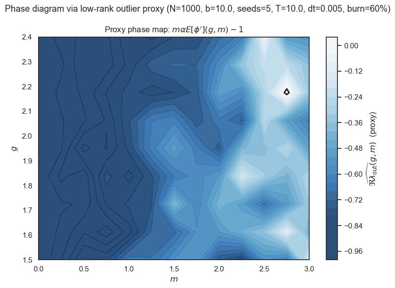
Figure 1: Phase diagram via low-rank outlier proxy. Filled contours show \(\widehat{\mathrm{Re}\lambda_{\mathrm{out}}}(g,m) = m(v^T \bar{A}(g,m)u)-1\) for \(N=1000\), \(b=10\). The black zero-level contour approximates the macroscopic stability boundary \(m^*(g)\). Brighter colors indicate larger (less stable) real parts of the predicted outlier. The map shows how increasing \(m\) eventually destabilizes the system, with sharper dependence near \(g \approx 2\).
Figure 1 shows the resulting phase map. The zero contour marks the transition: below it, the network is stable (fixed point); above it, stability is lost. The ridge around \(g \approx 2\) is a non-normal "most sensitive" region where small changes in \(m\) produce comparatively larger shifts in the outlier position.
validation: theory meets simulation
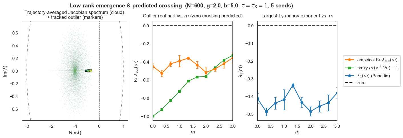
Does the theory actually work? Figure 2 tests the low-rank prediction at fixed \((g, b)\) by sweeping the rank-1 strength \(m\). For each \(m\), we:
- Time-average the Jacobian to obtain \(A_{\mathrm{avg}}\) and extract the outlier with maximal real part
- Record the largest Lyapunov exponent \(\lambda_1\) from the network dynamics
- Evaluate the scalar proxy \(m(v^T \bar{D} u)-1\) from the same run

Figure 2: Low-rank emergence and predicted crossing (rank-1). We fix \((N, g, b, \tau, \tau_S) = (600, 2.0, 5.0, 1, 1)\) and sweep the low-rank strength \(m\) (5 seeds). Left: Trajectory-averaged Jacobian spectrum (cloud), with the tracked outlier marked (X). Middle: Empirical \(\mathrm{Re}\lambda_{\mathrm{out}}(m)\) (orange, mean±SEM) versus the DMFT-style proxy \(m(v^T \bar{D} u)-1\) (green). Both curves approach 0 at similar \(m\), indicating the same predicted crossing. Right: Largest Lyapunov exponent \(\lambda_1(m)\) (blue, mean±SEM); it trends toward 0 near the crossing, consistent with loss of stability.
The empirical \(\mathrm{Re}\lambda_{\mathrm{out}}(m)\) and the proxy cross zero at similar \(m\) within error bars, and \(\lambda_1(m)\) approaches zero at the same location. This alignment validates our low-rank DMFT: the outlier controls the macroscopic stability boundary.
ablations: what matters?
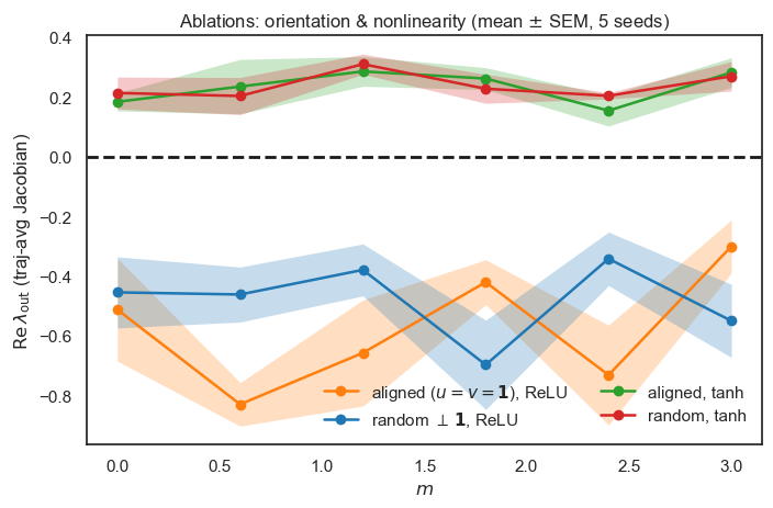
Does the phase boundary depend on the precise rank-1 orientation or the choice of activation function? Figure 3 shows that the sign change of \(\mathrm{Re}\lambda_{\mathrm{out}}(m)\) is preserved for both \(u=v=\mathbf{1}/\sqrt{N}\) (aligned with mean mode) and randomly oriented \(u, v \perp \mathbf{1}\), with only modest shifts in the threshold. Replacing ReLU by tanh slightly increases the effective gain (earlier crossing), consistent with the analytical dependence of the linearized gain \(\bar{D}\) on the nonlinearity.

Figure 3: Ablations: orientation and nonlinearity. Mean ± SEM over 5 seeds. We compare the low-rank direction aligned with the mean mode (\(u=v=\mathbf{1}/\sqrt{N}\)) versus random unit vectors orthogonal to \(\mathbf{1}\), and ReLU vs tanh. The zero crossing of \(\mathrm{Re}\lambda_{\mathrm{out}}\) persists under both alignment choices, confirming that the instability is a robust rank-1 effect rather than a special orientation.
The imaginary part remains near zero across conditions, indicating the dominant transition is a real-axis instability that governs stability/chaos via the sign of \(\mathrm{Re}\lambda_{\mathrm{out}}\).
interpreting the phase map: computational implications
What does the \((g, m)\) phase diagram tell us? Reading the map:
- Low \(g\), low \(m\): Stable fixed point. The network is quiescent, can store memories, but has no dynamics.
- Increasing \(m\): Structured modes become active. Can drive oscillations, enable rhythmic patterns and temporal encoding.
- High \(g\): Random bulk dominates. Chaos emerges, network is highly sensitive, good for exploration but hard to control.
- The sweet spot: Balance between structure and randomness. Enough structure for computation, not too much chaos.
Biologically, this suggests how networks might tune \((g, m)\) for different computational regimes. Task-specific networks might use higher \(m\) (more structure) for reliable, reproducible dynamics. Task-general networks might use higher \(g\) (more randomness) for flexibility and exploration.
closing: spectral blueprints for network design
We've developed a complete theoretical framework connecting low-rank structure to spectral outliers to phase transitions. The key results:
- Spectral theory: Finite-rank perturbations create isolated outliers via determinantal reduction and the isotropic resolvent limit
- Extended DMFT: Low-rank overlaps couple to mean-field equations, giving time-resolved stability analysis
- Fast proxy: Trajectory-averaged gain enables efficient phase diagram computation
- Phase boundaries: The real part of outliers marks fault lines where networks transition between dynamical regimes
Spectral outliers are the "blueprints" that control network behavior. Low-rank structure creates these blueprints in a controlled way. We can now predict and design network dynamics from connectivity structure. The theory provides a bridge between structure and function, showing how the spectral fingerprint of connectivity shapes the computational capabilities of neural networks.
Open questions remain: How do multiple low-rank terms interact nonlinearly? Can we design connectivity to achieve specific phase transitions? What about time-dependent low-rank structure (learning, plasticity)? These are directions for future exploration, but the foundation is now in place: we understand how structure creates spectral outliers, and how those outliers predict the fault lines in phase space.